I bought an electric car last month, which got me interested in my electric bill. I was surprised to find out that my electric company lets you export an hour-by-hour usage report for up to 13 months.
There are two choices of format: CSV and XML. I deal with a lot of CSV files at work, so I started there. The CSV file was workable, but not great. Here is a snippet:
"Data for period starting: 2022-01-01 00:00:00  for 24 hours"
"2022-01-01 00:00:00 to 2022-01-01 01:00:00","0.490",""
"2022-01-01 01:00:00 to 2022-01-01 02:00:00","0.700",""
The “Data for period” header was repeated at the beginning of every day. (March 13, which only had 23 hours due to Daylight Saving Time adjustments, also said “for 24 hours”.) There were some blank lines. It wouldn’t have been hard to delete the lines that didn’t correspond to an hourly meter reading, especially with BBEdit, Vim, or a spreadsheet program. But I was hoping to write something reusable in Python, preferably without regular expressions, so I decided it might be easier to take a crack at the XML.
Here is the general structure of the XML:
<entry>
  <content>
    <IntervalBlock>
      <IntervalReading>
        <timePeriod>
          <duration>3600</duration>
          <start>1641024000</start>
        </timePeriod>
        <value>700</value>
      </InvervalReading>
    </IntervalBlock>
  </content>
</entry>
Just like the CSV, there is an entry for each day, called an IntervalBlock. It has some
metadata about the day that I’ve left out because it isn’t important. What I care about
is the IntervalReading which has a start time, a duration, and a value. The start time
is the unix timestamp of the beginning of the period, and the value is Watt-hours.
Since each time period is an hour, you can also interpret the value as the average
power draw in Watts over that period.
XML is not something I deal with a lot day to day, so I had to read some Python docs, but it turned out very easy to parse:
from xml.etree import ElementTree
from datetime import datetime
import pandas as pd
import matplotlib.pyplot as plt

ns = {'atom': 'http://www.w3.org/2005/Atom', 'espi': 'http://naesb.org/espi'}
tree = ElementTree.parse('/Users/nathan/Downloads/SCE_Usage_8000647337_01-01-22_to_12-10-22.xml')
root = tree.getroot()
times = [datetime.fromtimestamp(int(x.text))
         for x in root.findall("./atom:entry/atom:content/espi:IntervalBlock/espi:IntervalReading/espi:timePeriod/espi:start", ns)]
values = [float(x.text)
          for x in root.findall("./atom:entry/atom:content/espi:IntervalBlock/espi:IntervalReading/espi:value", ns)]
ts = pd.Series(values, index=times)
The ns dictionary allows me to give aliases to the XML namespaces to save typing.
The two findall commands extract all of the start tags and all of the value tags.
I turn the timestamps into datetimes and the values into floats. Then a make them into
a Pandas Series (which, since it has a datetime index, is in fact a time series).
My electricity is cheaper outside of 4-9 p.m., so night time is the most convenient time to charge. I made a quick visualization of the last year by restricting myself from midnight to 4:00 a.m. andtaking the average of each day. Then I plotted it without lines and with dots as markers:
plt.plot(ts[ts.index.hour<4].groupby(lambda x: x.date).mean(), ls='None', marker='.')
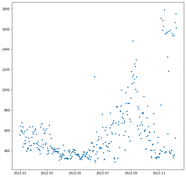
As expected, you see moderate use in the winter from the heating (gas, but with an electric blower). Then a lull for the in-between times, a peak in the summer where there is sometimes a bit of AC running in the night, another lull as summer ends, and then a bit of an explosion when I started charging the car.
For now, I am actually using a 120 V plug which can only draw 1 to 1.5 kW and is a slow way to charge a car. Eventually I will get a 240 V circuit and charger, increase the charging speed 5x, and have even bigger spikes to draw.